The Core Idea
The Central Limit Theorem, usually called the CLT, is one of the most important ideas in statistics because it explains why sample averages behave in a surprisingly regular way.
Many people first meet the theorem as a difficult sentence. But the real idea is much simpler: even if the original data is messy, uneven, or not normally shaped, the averages of many repeated samples tend to form a normal-looking pattern.
In plain words, raw data can be wild, but averages calm things down. When you keep taking samples of the same size and compute the average each time, those averages usually start gathering around the true population mean.
This is why the theorem is powerful. In real life, we usually do not know the whole population. We work with samples. CLT tells us that if the sample size is reasonably large, the sampling distribution of the sample mean becomes approximately normal.
That sentence has three important parts: sampling distribution, sample mean, and approximately normal.
Sampling distribution does not mean the original data table. It means the pattern formed by a statistic after repeating sampling many times. Here the statistic is the sample mean. So CLT is not mainly about individual observations. It is about the behavior of averages of samples.
This is the most common confusion: students think CLT says the original population becomes normal. It does not. The population may be skewed, lumpy, strange, or uneven. CLT says the distribution of sample means becomes approximately normal as the sample size grows.
Suppose incomes in a city are very skewed because a few people earn much more than everyone else. Individual incomes are not normal at all. But if you repeatedly take samples of, say, 40 people and compute the average income each time, those sample averages tend to behave much more smoothly.
Why does this happen? Because extreme highs and lows partly cancel out when averaged. One person may be unusually high, another unusually low, and the average pulls them together. A single data value can jump around a lot. An average is more stable.
CLT is also connected to two numbers: the population mean and the standard error. The center of the sampling distribution of the sample mean is the population mean. The spread of that sampling distribution is: sigma / sqrt(n) where sigma is the population standard deviation and n is the sample size.
This formula tells us something important: when sample size gets larger, the denominator sqrt(n) gets larger, so the spread gets smaller. That means larger samples produce averages that are more tightly clustered around the true mean.
So CLT gives us two strong comforts:
1. The averages become normal-like.
2. The averages become less spread out when sample size increases.
Another common confusion is about the phrase "sample size 30". Many textbooks casually say that n = 30 is enough. Treat that as a practical rule of thumb, not a magical law. If the original population is already fairly regular, smaller samples may work well. If the population is extremely skewed or has heavy outliers, a bigger sample may be safer.
CLT matters because many statistical methods depend on normality, at least approximately. Confidence intervals, hypothesis tests, and many inferential tools become usable because CLT helps justify normal-based reasoning for sample means.
Here is the essence in one clean contrast:
Population distribution
= how individual values behave.
Sampling distribution of the mean
= how repeated sample averages behave.
CLT speaks mainly about the second one.
If you remember only one mental picture, use this: imagine scooping water from a shaky river. A single drop may move wildly, but the average level in many cups becomes much more predictable. CLT is the mathematics behind that calmness.
The theorem does not say "everything becomes perfect." It says that with repeated sampling and a large enough sample size, the sample mean becomes predictable enough for us to use normal tools sensibly.
So the basic essence of the theorem is this: averaging creates order out of randomness.
Examples and Intuition
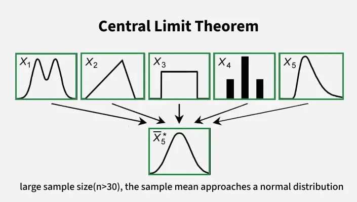
Source: Google Images
Example 1: One student vs class average
Suppose a class has some very high marks, some low marks, and many in the middle.
A single student's mark can vary a lot.
But if you take groups of 40 students and compute the average mark of each group,
those group averages will vary much less than individual marks.
This is the spirit of CLT.
Example 2: Skewed population, calmer averages
Imagine shop purchase amounts.
Most customers spend a little, a few spend a lot.
So the raw data is right-skewed.
Now repeatedly take samples of 50 bills and compute the average bill amount each time.
The shape of those averages will usually be much more balanced and bell-like than the raw purchase amounts.
Example 3: Dice average
A single die roll can only be 1, 2, 3, 4, 5, or 6.
That is not a normal distribution.
But if you roll 30 dice, compute the average, and repeat this experiment many times,
the pattern of those averages begins to look approximately normal around 3.5.
This example is useful because it shows the theorem clearly: the original data is not normal, but the sample means move toward a normal shape.
Example 4: What "centered at the true mean" means
Suppose the population mean height is 160 cm.
Then the mean of all possible sample means is also 160 cm.
Some sample averages may be 158, some 161, some 162,
but taken together, they center around the real population mean.
Example 5: Why larger samples help
Take samples of size 5 and compute averages.
Those averages may jump around a fair amount.
Now take samples of size 100 and compute averages.
These new averages will be much more tightly packed near the true mean.
So larger sample size means greater stability.
Example 6: Standard error in plain English
Standard deviation tells us how much individual values vary.
Standard error tells us how much the sample mean varies from sample to sample.
If standard error is small, the sample mean is more dependable.
Example 7: A tiny numerical illustration
Suppose population mean = 50 and population standard deviation = 20.
| Sample size n | Standard error = 20 / sqrt(n) |
|---|---|
| 4 | 10.00 |
| 16 | 5.00 |
| 25 | 4.00 |
| 100 | 2.00 |
As n grows, standard error falls. That means sample means become less scattered. This table alone explains a large part of why CLT matters in practice.
Example 8: What CLT does not say
It does not say every sample mean equals the population mean exactly.
It does not say the original data must be normal.
It does not say n = 30 always solves every problem.
It does say that repeated sample means tend toward a normal pattern and become more stable as n increases.
Example 9: Why this helps confidence intervals
If sample means behave approximately normally, then we can estimate how far a sample mean is likely to be from the true mean.
That is the backbone of many interval estimates and significance tests.
Without this normal-like behavior, inferential statistics would be much harder to use.
Example 10: The three-layer picture
Layer 1: Individual observations may be messy.
Layer 2: Sample means are smoother.
Layer 3: Large-sample methods become possible because those sample means are approximately normal.
This three-layer picture often removes most of the confusion.
Quick memory sentence
Raw values may be irregular.
Repeated sample averages become regular.
That regularity is the heart of the Central Limit Theorem.
One final plain-language summary
If you keep drawing reasonably large samples from the same population and average each sample,
the collection of those averages will usually form a bell-shaped pattern around the true mean,
and bigger samples make that bell tighter.